This is the course notes I took when studying Introduction to Corporate Finance, offered by Wharton on Coursera.

Time Value of Money

The intuition of time value of money comes from currency: how much money do I have with 100 dollars and 100 euros? It cannot be answered unless one currency is converted into a common (base) currency using the exchange rate.

Likewise, money received/paid at different times is like different currencies: money has a time unit. It must be converted to common/base unit to aggregate and we need an exchange rate for time. The tool is time line and discount factor.

Time line lays out different time periods (unit could be arbitrary). Typically we refer to time period $0$ as today or now or the point at which we’re answering the question. Underneath the time line we lay out the cash flows for each period, denoted as $CF_n$ where $n$ is the time period.

Lesson: Get in the habit of placing cash flows on a time line.

Lesson: Never add/subtract cash flows received at different times. It might be OK for cash flows within a short period of time.

The discount factor, $(1+R)^t$, is our exchange rate for time, where $t$ is time periods into future ($t > 0$) or past ($t < 0$) to move CFs.

Definition: $R$ is the rate of return offered by investment alternatives in the capital markets of equivalent risk. A.k.a., discount rate, hurdle rate, opportunity cost of capital.

To determine $R$, consider the risk of the cash flows that you are discounting.

Using the tool we could move cash flows in time via discounting and compounding.

Discounting

Discounting is the process of moving CFs back in time ($t < 0$). Present value, $PV_t(\bullet)$ of $CF_i$ is discounted value of $CF_i$ as of $t$. Generally we look at PV at time $0$ (at present), so $PV_0(CF_i)=CF_i\times (1+R)^{-i}$.

Once cash flows are moved to the same time, we can add them up. For example, a cash flow of 100 dollars per year in the next 4 years can be interpreted as:

We need $354.60 today in an account earning 5% each year so that we can withdraw $100 at the end of each of the next four years.
The present value of $100 received at the end of each of the next four years is $354.60 when the discount rate is 5%.
Today’s price for a contract that pays $100 at the end of each of the next four years is $354.60 when the discount rate is 5%.

We need to call out that we assume the discount rate $R$ is constant over time, but it may not be the case. So in general present value as of time $s$ of a cash flow at time $t > s$, $PV_s(CF_t)$, tells us the value of future cash flows, or the price of a claim to those cash flows.

Compounding

Compounding moves CFs forward in time ($t > 0$). Future value, $FV_t(\bullet)$ of $CF_i$ is compounded value of $CF_i$ as of $t$. $FV_s(CF_t)=CF_t(1+R)^{s-t}$.

Compounding tells us the future value of cash flows.

We can use discounting and compounding at the same time to calculate the value/price of a cash flow, as long as the time unit is the same.

Examples of Cash Flows

Here are a few examples of cash flows and their present values.

An annuity is a finite stream of cash flows of identical magnitude and equal spacing in time. E.g., Savings, vehicle, home mortgage, auto lease, bond payments.

\[PV=CF\times\frac{1-(1+R)^{-T}}{R}\]

A growing annuity is a finite stream of cash flows that grow at a constant rate $g$ and that are evenly spaced through time. E.g., Income streams, savings strategies, project revenue/expense streams.

\[PV=\frac{CF}{R-g}\big(1-\big(\frac{1+R}{1+g}\big)^{-T}\big)\]

An perpetuity is an infinite stream of cash flows of identical magnitude and equal spacing in time.

\[PV=\frac{CF}{R}\]

A growing perpetuity is an infinite stream of cash flows that grow at a constant rate $g$ and that are evenly spaced through time. E.g., Dividend streams (companies last indefinitely).

\[PV=\frac{CF}{R-g}\]

Assuming the first cash flow arrives one period from today, and growth rate must be less than the discount rate.

Taxes

Taxes reduce our return. The after-tax return $R_t=R\times(1-t)$ where $R$ is the nominal return and $t$ is the tax rate.

Inflation

Unlike taxes, inflation won’t affect the money we earn, but what we can buy with the money. The real discount rate (adjusted by the expected inflation rate $\pi$), $RR$, is calculated as

\[1+RR=\frac{1+R}{1+\pi}\approx R-\pi\]

Ideally, we want to adjust our future cash flows with inflation rate to preserve purchasing power. But

PV of nominal CFs at nominal discount rate = PV of real cash flows at real rate.

Interest Rates

Interest rates are quoted in rates:

Rate, or APR (Annual Percentage Rate): measurement of amount of simple interest (i.e., without compounding) earned in a year. But APR is not typically what we earn or pay.
APY (Annual Percentage Yield) or EAR (Effective Annual Rate): measurement of actual amount of interest earned/paid in a year.

EAR is a discount rate, so it is what matters for computing interest and discounting cash flows. APR is not a discount rate. APR is a means to an end. We use it to get a discount rate (e.g., EAR).

\[EAR = \big(1+\frac{APR}{k} \big)^k-1=(1+i)^k-1\]

Where $k$ is the number of compounding periods per year, and $i$ is the periodic interest rate, or periodic discount rate.

Lesson: If you discount cash flows using EAR, then measure time in years. If you discount cash flows using periodic interest rate, then measure time in periods.

Term Structure

So far we have assumed the interest rate is constant over time. However, in most cases, the interest rate increases when the investment term increases. The Term Structure is the relation between the investment term and the interest rate. And the Yield Curve is a graph of the relation between the investment term and the interest rate.

A yield, $y$, is the one discount rate that when applied to the promised cash flows of the security recover the price of the security. It can be computed from

\[Price=\frac{CF_1}{(1+y)}+\frac{CF_2}{(1+y)^2}+\frac{CF_3}{(1+y)^3}+...+\frac{CF_T}{(1+y)^T}\]

To build the yield curve, simply compute the yield for securities of different maturities. Yield Curves can move around a lot. And the relationship between short-term rates and long-term rates can change. The upward sloping curve (short-term rates are lower than the long-term rates) suggest that the expectation of future interest rates is higher, and vice versa.

Yield curves can be built for different types of securities. Treasury Yield Curves show the relation between interest rates on risk-free loans and loan maturity. Yield curves for different securities can be used to compare interest rates based on risks.

Lesson: Yields vary by maturity and risk.

Therefore, when discounting future cash flows, the discount rate can vary by a lot based on the time periods.

Note, all of these interest rates are referred to as spot rates. The spot rate is the interest rate for a loan made today.

Discounted Cash Flow Analysis

Discounted cash flow analysis is a mean for decision-making based on finance. The intuition of decision making is to undertake those actions that create value, those in which the benefits exceed the costs. While costs and benefits can arrive at different time, we can compare their present values for decision-making.

Lesson: The NPV (Net Present Value) Decision Rule says accept all projects with a positive NPV and reject all projects with a negative NPV.

\[NPV = PV(Benefits) - PV(Costs) = FCF_0+\frac{FCF_1}{(1+R)}+\frac{FCF_2}{(1+R)^2}+...+\frac{FCF_T}{(1+R)^T}\]

$FCF$ stands for free cash flow. NPV is a decision rule that quantifies the value implications of decisions. It is used in conjunction with other rules, such as Internal Rate of Return (IRR) and Payback Period rule.

Free Cash Flow

NPV contains two components:

Free cash flow;
Discount rate.

FCF is defined as

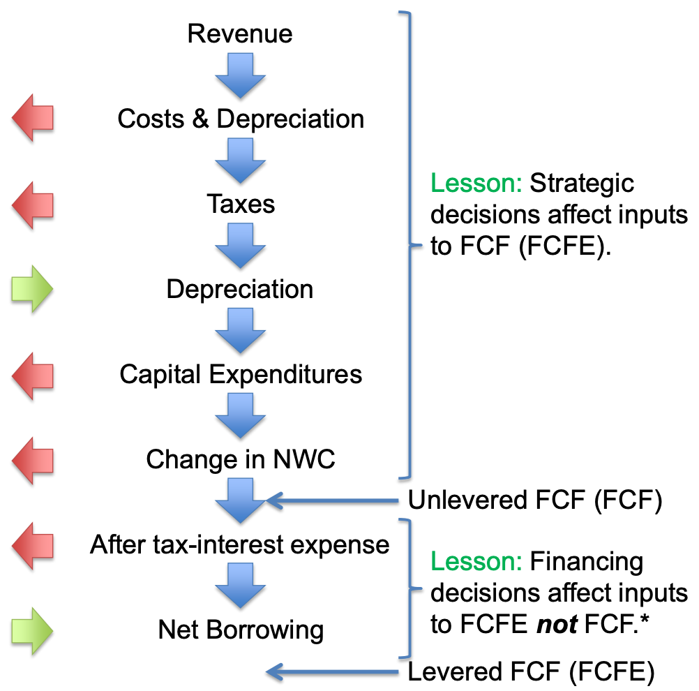
\[\begin{align}\begin{aligned} \text{FCF}=&(\text{Revenue} - \text{Cost} - \text{Depreciation})\times(1-t_C) \\ +& \text{Depreciation} - \text{Capital Expenditures} \\ -& \text{Change in Net Working Capital} \end{aligned}\end{align}\]

The first line, $(\text{Revenue} - \text{Cost} - \text{Depreciation})\times(1-t_C)$, is called Unlevered Net Income, Net Operating Profit After Taxes (NOPAT), or Earnings Before Interest After Taxes (EBIAT). While depreciation is not money leaving the company, it is tax deductible so it must be subtracted. $t_C$ is the marginal tax rate.

Net Working Capital (NWC) is current assets subtracted by current liabilities. Current asset is the sum of cash, account payable, and inventory, and current liabilities is mostly account payable. NWC consists of stock variables so we calculate FCF using the change in NWC.

Lesson: FCF is the residual cash flow left over after all of the project’s requirements have been satisfied and implications accounted for.

Lesson: FCF is the cash flow that can be distributed to the financial claimants (e.g., debt and equity) of the project or company.

Lesson: FCF is not the same as accounting cash flow from the statement of cash flows (SCF) but we can derive FCF from the SCF.

Lesson: FCF is more precisely unlevered free cash flow to distinguish it from free cash flow to equity (FCFE) or levered free cash flow.

\[\text{FCFE} = \text{FCF} – \text{Interest} \times (1 – t_C) + \text{Net Borrowing}\]

Net borrowing is borrowing after any debt repayment.

Lesson: FCFE is residual cash flow left over after all of the project’s requirements have been satisfied, implications accounted for, and all debt financing has been satisfied.

Debts are taken care of between FCFE and FCF because they are senior claimants than equity.

Lesson: FCFE is the cash flow that can be distributed to the shareholders (i.e., equity) of the project or company.

Lesson: FCFE is more precisely levered free cash flow because it is affected by the choice of leverage (i.e., debt).

An illustration among these terms is below: Free Cash Flow

Forecast Drivers

Forecast drivers are assumptions used to forecast each component in the FCF.

$\text{Revenue}=\text{Market Size}\times\text{Market Share}\times\text{Price}$ and each component can be forecasted separately.
$\text{Cost}=\text{Cost Margin}\times\text{Revenue}$, such as COGS (cost of goods sold).
$\text{Net Working Capital} = \text{Cash} + \text{Inventory} + \text{AR} - \text{AP}$, in which
- Cash is used for manufacturing and pay employees, as a percentage of these items;
- Inventory is quantified by days that products sit in the warehouse (as a percentage in a year of COGS), plus the liquidation value for the excess inventory.
- Account Receivable and Payable are days receivable and payable are paid (as a percentage in a year of sales/COGS). Most of sales are done via credits.

While accurate forecasting is nearly impossible, the point of DCF is to provide a framework for the discussion and analysis on relevant issues. Successful valuation (i.e., decision making) depends critically on input from non-finance personnel, because many forecasts depend on the business, not finance.

Forecasting free cash flows is a matter of converting our forecast drivers into dollar forecasts.

Other free cash flow considerations:

Opportunity cost: alternative uses of resources;
Project externalities: cannibalization of products within the same company, spillovers (benefits/costs to other projects);
Sunk costs: we should ignore them;
Other non-cash items: e.g., amortization, stock options;
Salvage values: assets do not disappear, they can be sold;
Execution risks of projects;
Cash flow frequency.

Decision Criteria

Once the discounted cash flow analysis is completed (i.e., we have our FCF), we can use it to make decisions.

Calculate the NPV and use NPV rule as the decision criteria.
Calculate the internal rate of return (IRR), the one discount rate such that the net present value of the project’s free cash flows equals zero.

Lesson: The IRR Rule says accept all projects whose $IRR > R$, reject all projects whose $IRR < R$.

The IRR rule means the project generates higher return ($IRR$) than cost of capital (hurdle rate $R$). But the IRR rule has some shortcomings (more later).
Compute the payback period $pp$, of a project is the duration until the the cumulative free cash flows turn positive.

Lesson: The Payback Period Rule says accept all projects with payback period shorter than some threshold.

The Payback Period Rule has several shortcomings:
1. It ignores the time value of money and risk of cash flows. The mitigation is to use discounted payback period, $dpp$, of a project is the duration until the the cumulative discounted free cash flows turn positive.
2. It ignores cash flows after cutoff leading to myopic decision making. If the cash flow goes deep in negative before the payback period, we may be forced to end the project prematurely and will not see the break-even positive cash flow at a later time.
3. Does not help in choosing among projects with similar payback periods.

To summarize, NPV rule is unambiguously the best but others are also informative.

Sensitivity Analysis

Sensitivity analysis is an integral part of any valuation. It helps us answer the key questions in valuation:

Where value is created and destroyed?
What are the key value drivers?
What is the risk exposure?
How robust is the profitability of the project?

Break Even Analysis finds the parameter value that sets the NPV of the project equal to zero holding fixed all other parameters. It can identify parameters with large margin of error, and potentially important ones that large deviations in assumptions could lead to destructive results.

Lesson: Break Even Analysis is a partial equilibrium analyses that assume parameters are independent of one another.

Comparative statics quantifies the sensitivity of the valuation to variation in a parameter holding fixed all other parameters. If the range of each parameter (from worst case to the best case) can be identified, we can calculate the corresponding NPV for the worst case and the best case and answer the question: does the valuation vary sensibly with variation in the parameters?

The next question is what is the elasticity of the valuation with respect to each parameter? How does valuation change relative to parameter change?

\[\text{Elasticity}=\frac{\%\text{ Change in NPV}}{\%\text{ Change in Parameter}} = \frac{\Delta NPV}{\Delta P}\cdot\frac{P}{NPV}\]

By looking for parameters with high elasticity, we can identify important parameters.

Lesson: Comparative statics implicitly assumes parameters are independent of one another.

Scenario Analysis quantifies the sensitivity of the valuation to variation in multiple parameters. Commonly, when two parameters change, we can build a two-way sensitivity table to quantify the change in NPV according to variations in them.

Simulation Analysis performs the valuation for a large number of simulated parameter values (i.e., scenarios). One way to do it is to draw random values for all parameters within the range from worst case to the best case, calculate the NPV and draw the distribution of NPV. If the majority of NPV is positive, it means the possibility of getting it right is high. However, some times parameters are not independent from each other and such drawing creates unreasonable scenario (e.g., price vs. quantity), but it is still a good practice without going into details of valuation.

Return on Investment

The IRR rule is another popular decision making rule other than the NPV rule.

Lesson: The IRR rule leads to the same decisions – accept or reject – as the NPV rule if all negative cash flows precede all positive cash flows.

However, when the signs of cash flows are not proper, it could lead to multiple IRRs or imaginary (mathematically) IRRs, rendering it useless.

In addition, the IRR Rule can mislead decision making when comparing projects even when cash flow signs are proper. This is because IRR does not account for differences in scale (Would you rather earn 100% on a $1 investment or 10% on a $1,000,000 investment?)

Lesson: IRR increased because initial investment fell more than future cash flows. Intuition: Small payoffs on a smaller investment can generate very large returns because of division by small numbers.

Lesson: Front-loaded CFs (higher CF initially) can increase IRR.

Thus, IRR should be used in conjunction with NPV analysis.